CS194 Project 7A: Image Warping and Mosaicing

Rohan Chitnis

(Skip to bells and whistles section.)

Background

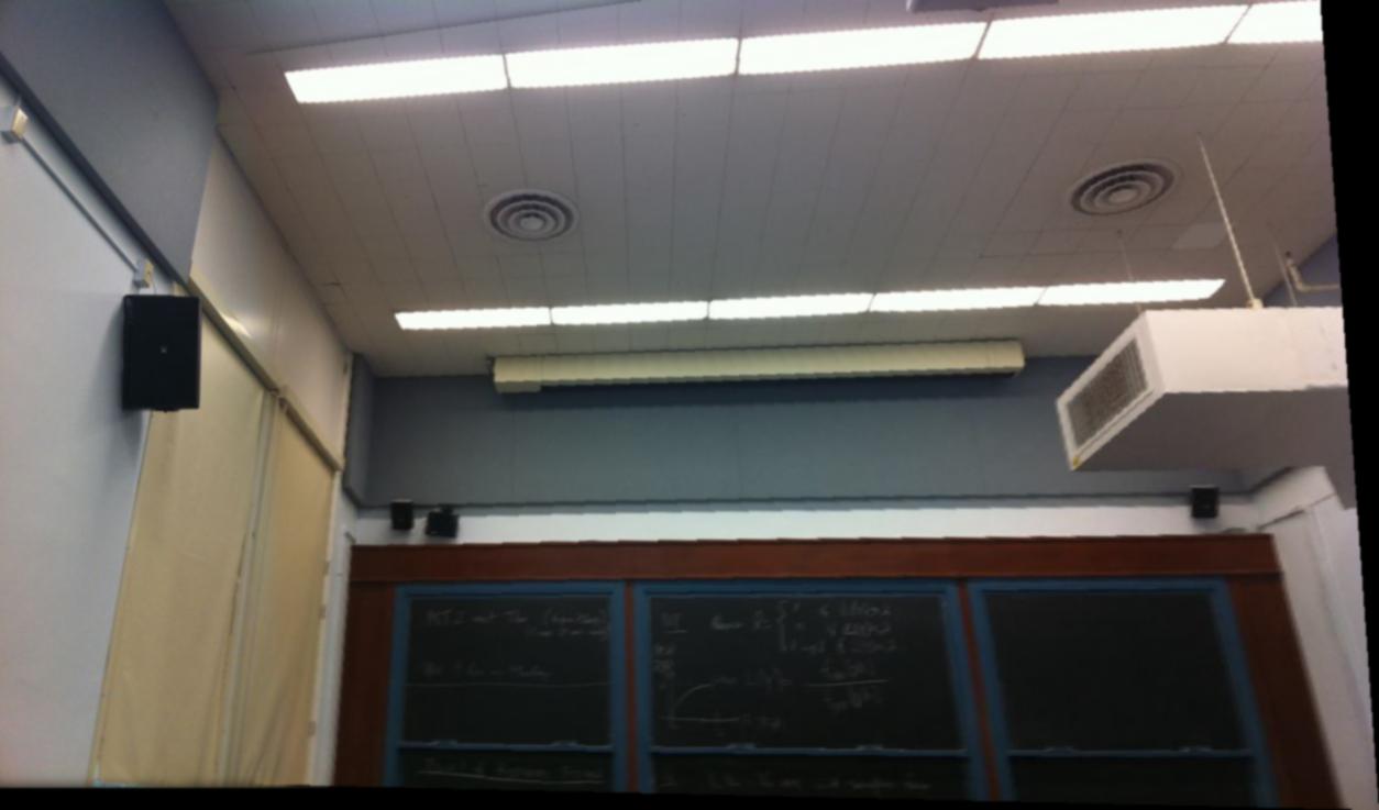
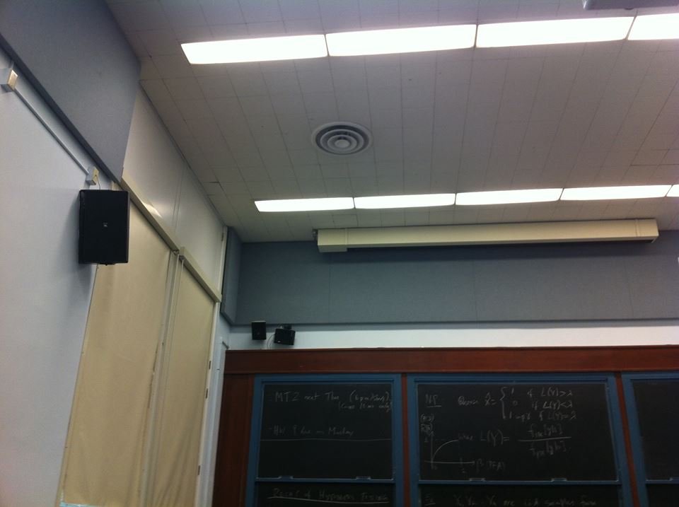
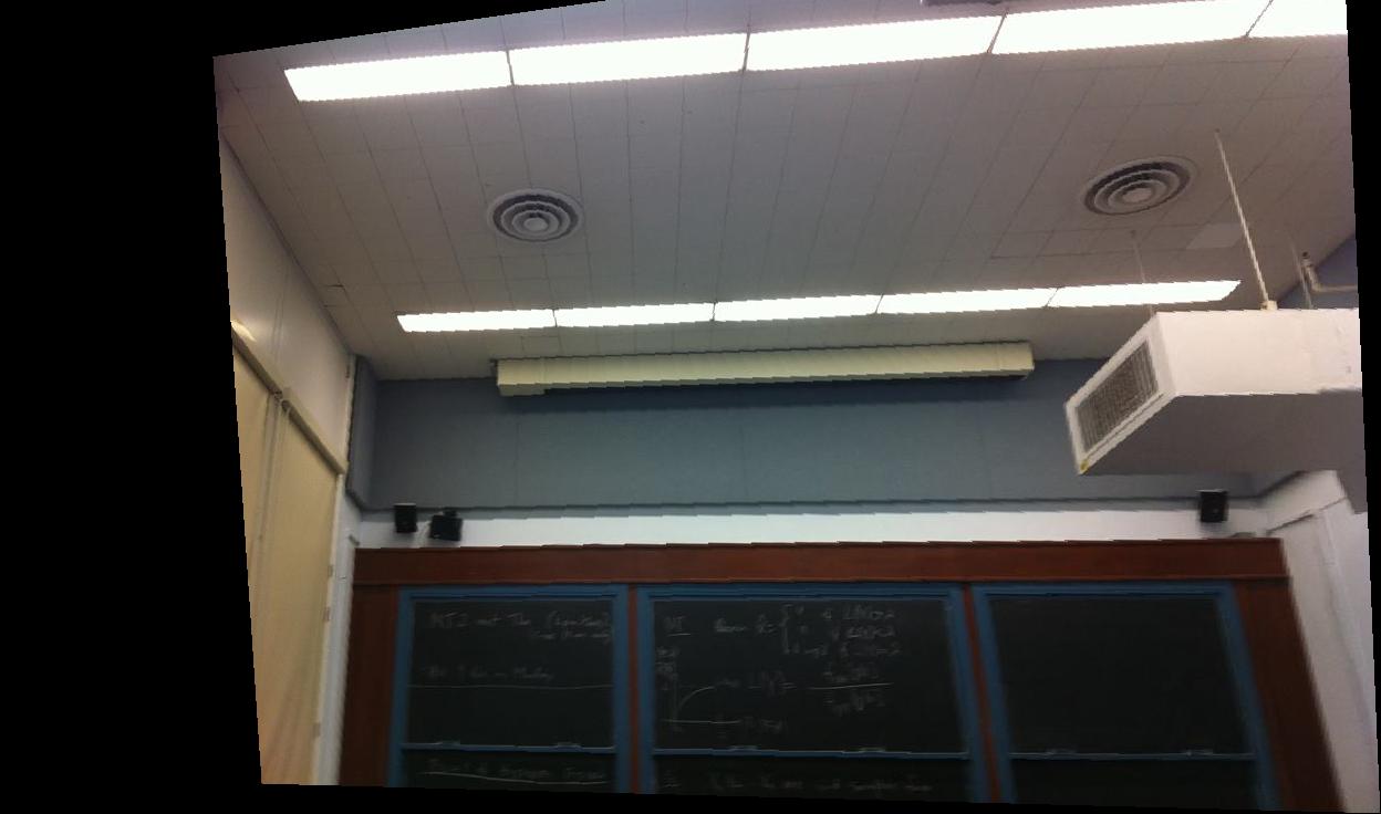
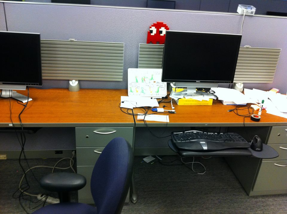
For this project, we used homography transformations to create warps between images, and subsequently create mosaics from stitching together a collection of images which represent a panomaric view of a scene. For simplicity and consistency, my implementation warps all images to the first one, so if the images are provided left-to-right as in my examples, all images are warped to the left-most one. First, I select control points matching each image to the first one, and find a homography transformation between them, by setting up a simple linear system of equations dependent on the number of control points provided. The resulting matrix has a 1 on the lower-left corner, used as a scaling factor because we are working with homogenous coordinates in each image. Next, I go through each image which is not the first and warp it to the first (which remains unwarped), growing my mosaic one-by-one. The warping occurs as follows: left-multiply the corners of the image by the transformation matrix to determine the size of the output image, then do inverse warping as done in project 5 to fill in the output pixels, interpolating where appropriate. I blend together the mosaics using three methods: a naive average, linear (alpha) blending, and Gaussian and Laplacian stacks (implementation taken from my project 3).

Homographic Transformations

I will illustrate homographic transformations now!

The original 2 images of a lecture hall in Berkeley. An important note is that only a rotation separates the image views, because translation breaks the homographic transform.

Left: Warping the left image to match the right one's shape and viewpoint. Notice that it now looks as if the left picture were taken from the same point of view as the right one!

Right: Warping the right image to match the left one's shape and viewpoint. Notice that it now looks as if the right picture were taken from the same point of view as the left one! This is very evident if you look at features of the ceiling.

Image Rectification

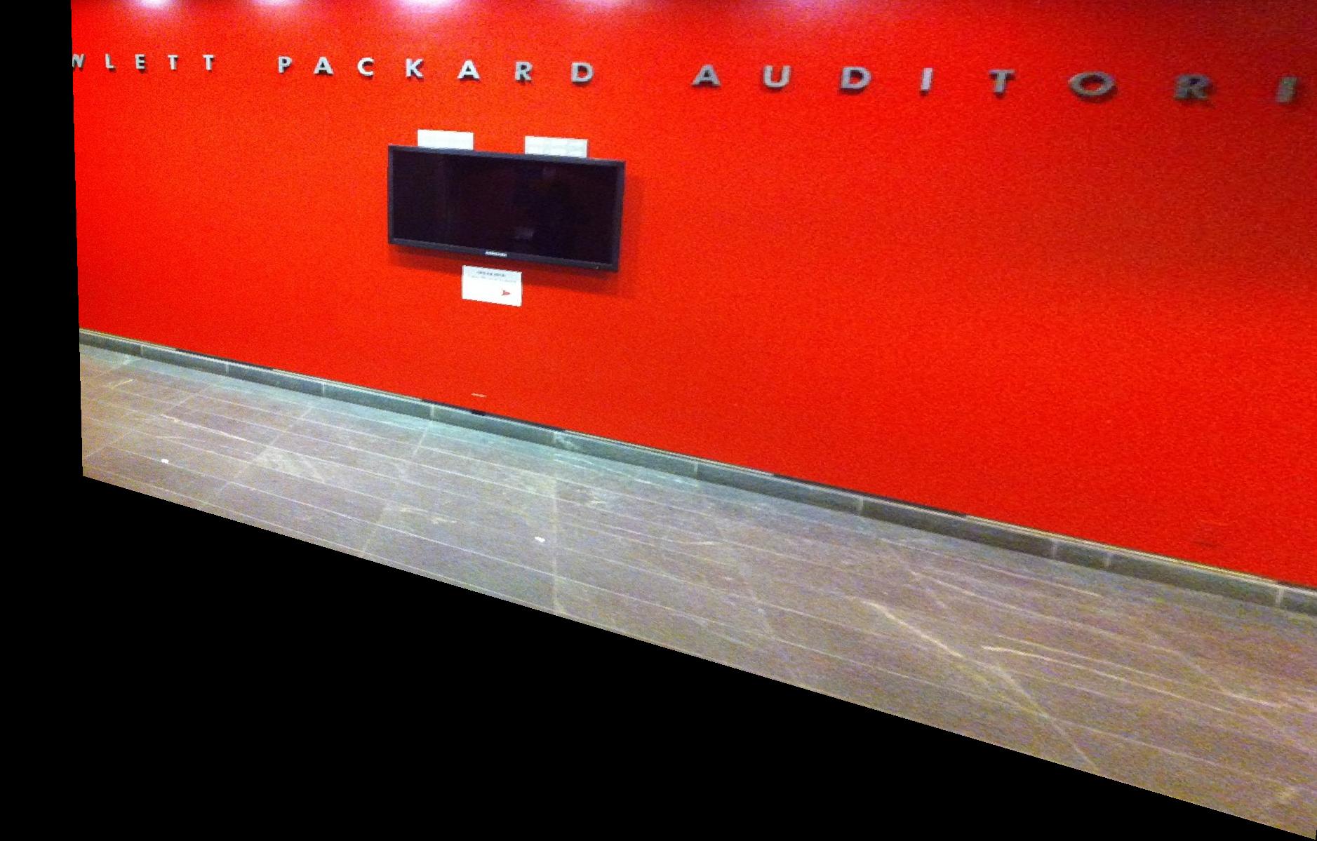
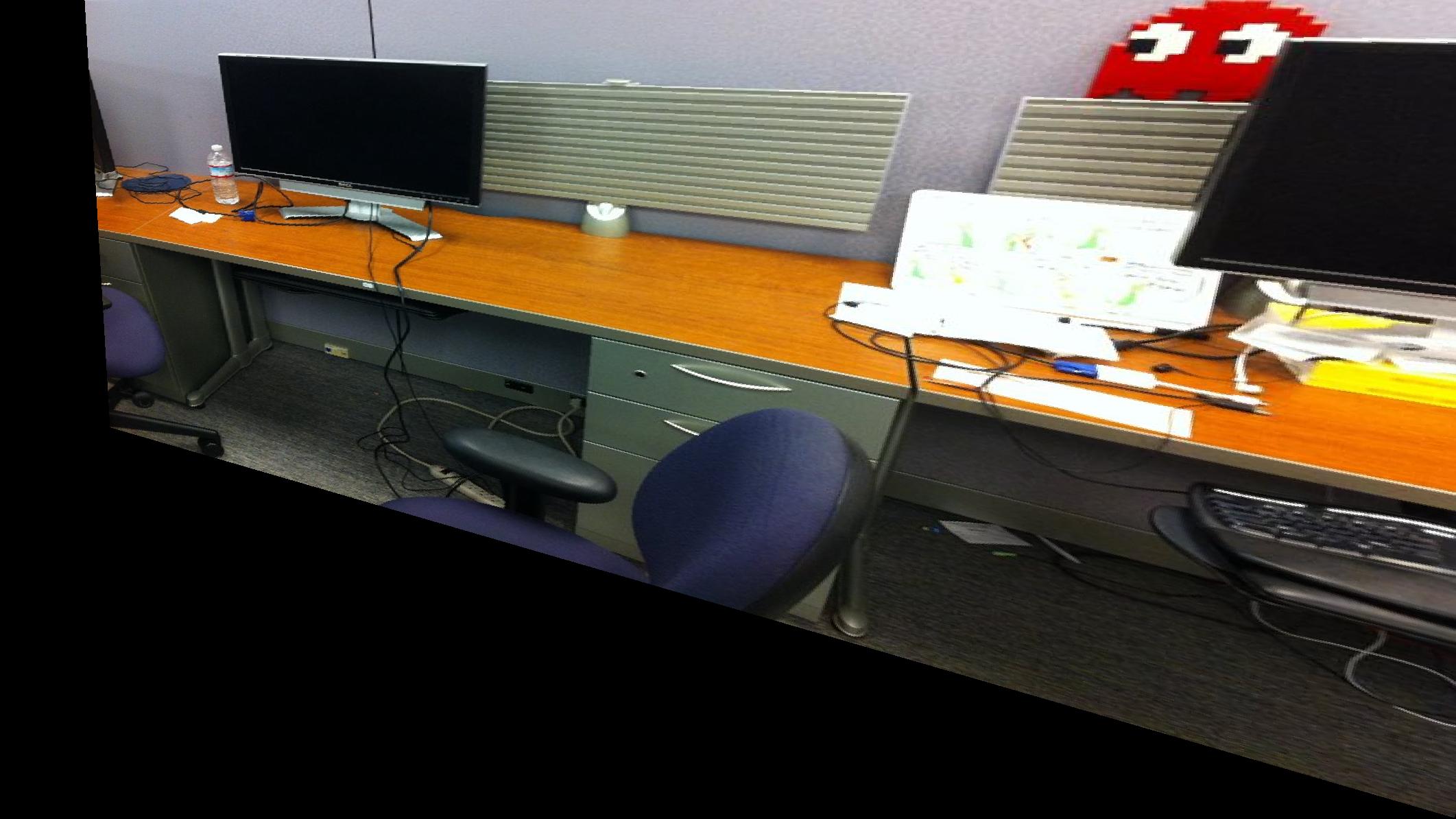
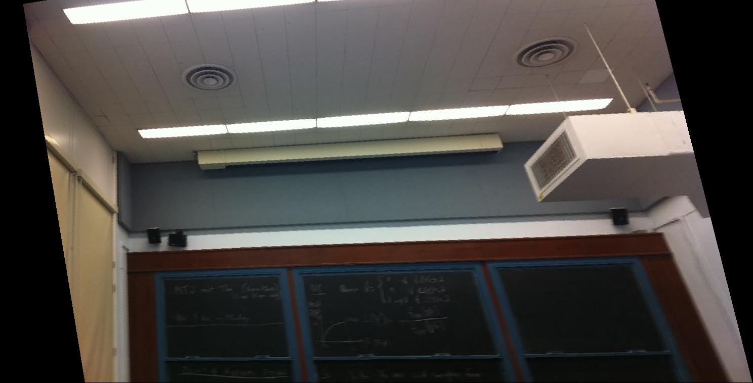
I am now able to easily rectify an image by transforming a portion which I want to be a rectangle into a rectangle. Here are some examples!

Left: I had a midterm that day, so it's only appropriate that I let the blue book serve a dual purpose. This is the original image.

Middle: Image rectification, by warping the blue book edges to make it a rectangle. It's amazing how this technique allows us to guess at what the top-down view of something looks like!

Right: Same rectified image, cropped for increased viewing pleasure.

A similar set of images as before, but this time with an object placed on top of the paper! I wanted to see what would happen with the object; it got transformed quite realistically. You can definitely see less of its bottom blue portion in the warped image, as expected. Perhaps the most amazing thing about this rectification is that the words on the paper are actually slightly more readable after the warping, even though the information could not be any different!

Here is a failed example of rectification, because the object on the paper was too tall. Obviously, a top-down view into the glass is not possible because the original image does not contain the information about how the glass looks on the inside. Also, the glass blocks the back portion of the paper, which thus cannot be present in the warped image either.

Mosaic Creation

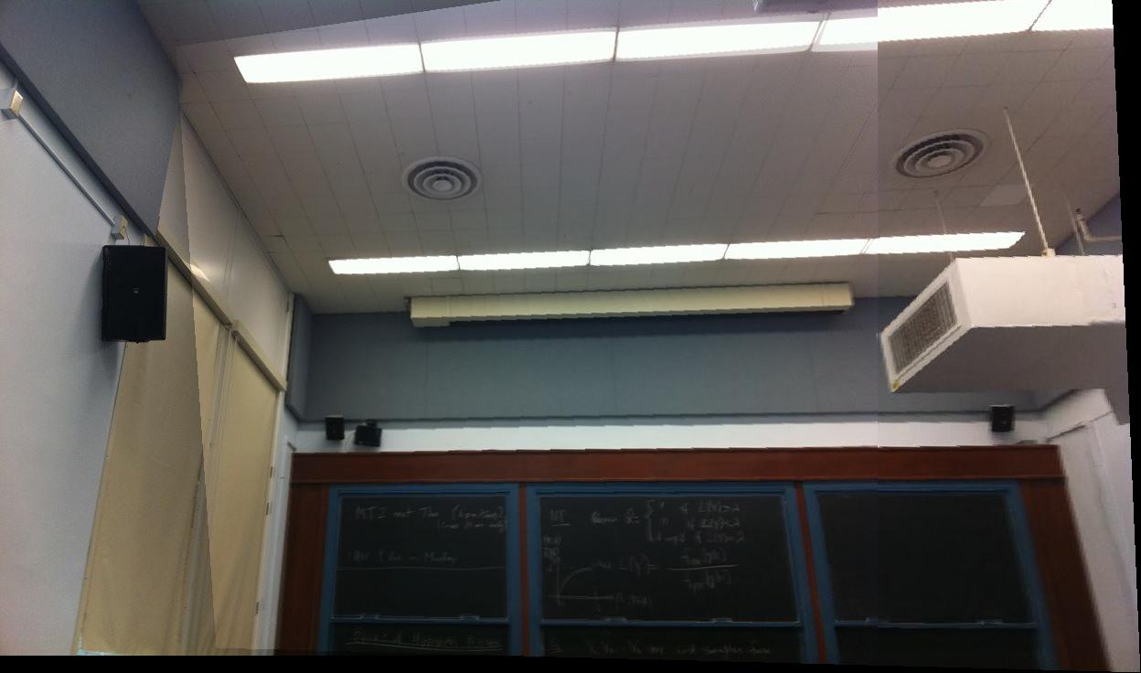
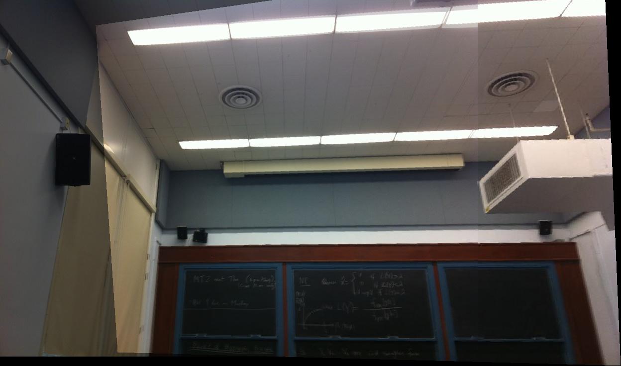
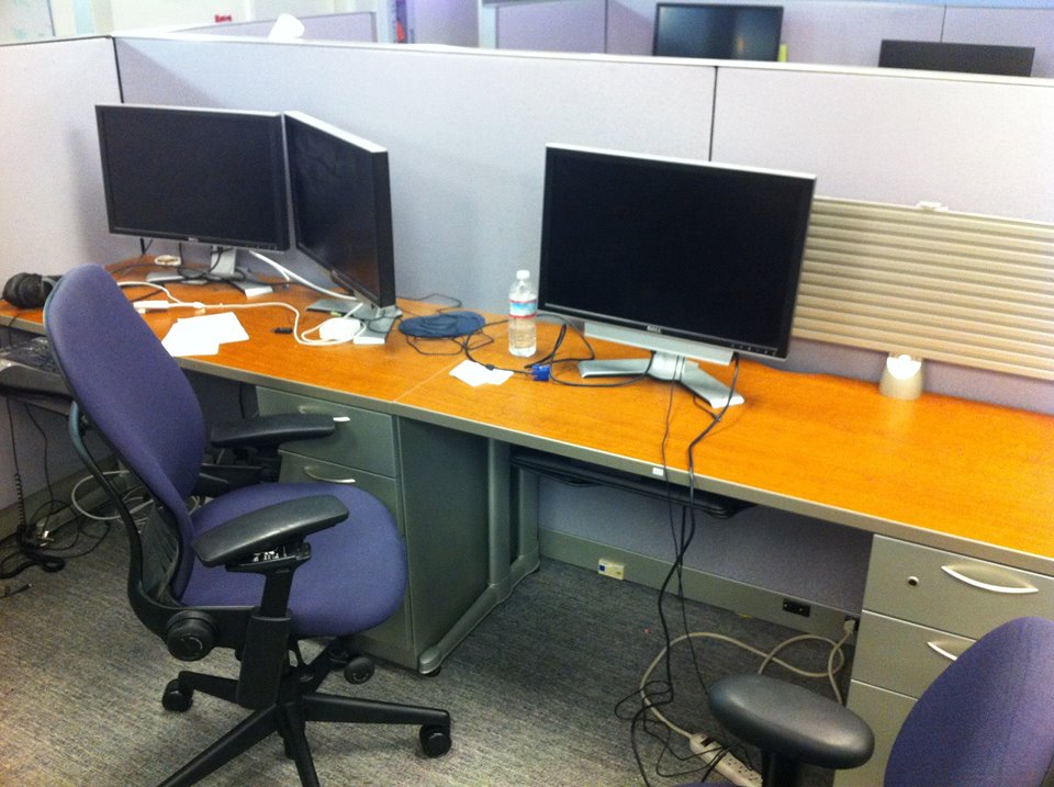
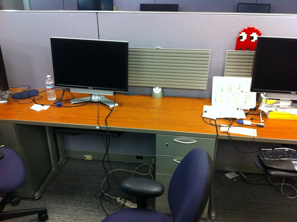
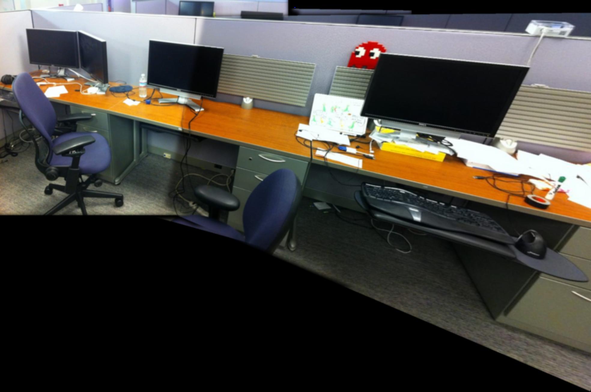
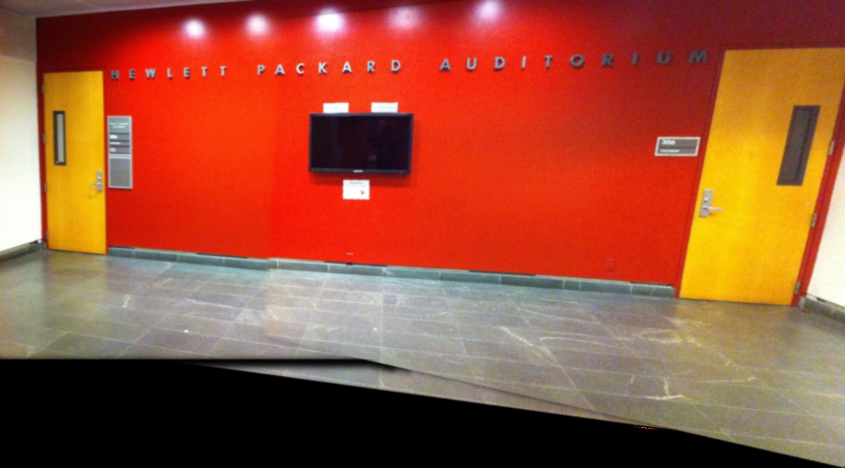
As described in the Background section, I warp each image to the first one, growing my mosaic one image at a time, and blending together using three methods: a naive average, linear (alpha) blending, and Gaussian and Laplacian stacks with size 3. Here are results for all cases.

The original 2 images of a lecture hall in Berkeley.

Left: The resulting mosaic, creating using the steps described in the Background section, blended with Gaussian and Laplacian stacks. The seam is nearly flawless using this blending method.

Right: The resulting mosaic, blended using linear blending, with alpha interpolated linearly from the center of the image going toward the ends. The result is better than that of the naive averaging (below), for obvious reasons, but still cannot match the quality of using Gaussian and Laplacian stacks.

The resulting mosaic, blended using naive averaging. Clearly, the quality is not good due to the obvious seams.

Today, I went to watch the premiere of some Disney movie which turned out to be bad. I used the opportunity to snap some pictures of Shattuck cinemas, my set of off-campus images!

Left: The resulting mosaic, blended with Gaussian and Laplacian stacks. Again, a barely noticeable seam. The only issue here is a tone difference in the original images. To see the power of the transformation here, it's best to focus on the building above the theater, as the warping is very evident for it. Compare the building's orientation here to that in the second original image.

Right: The resulting mosaic, blended using linear blending. Again, better than naive averaging (below) but worse than using stacks. Although the tone difference is smoothed away, the seams are more apparent.

The resulting mosaic, blended using naive averaging. Again, bad seams so low quality.

Moving from 2 to 3 images in the mosaic now! Here are the original images of a desk at my research lab.

Mosaic results, similar to before, using Gaussian and Laplacian stack blending. Notice that elements of all 3 images are present in the final mosaic. Again, some tone differences in the original images manifest themselves slightly.

Original images outside HP Auditorium!

Mosaic results, similar to before, using Gaussian and Laplacian stack blending. As before, notice that elements of all 3 images are present in the final mosaic. It really seems as though the entire mosaic image were taken from the point of view of only the left-most image! This is truly astounding to look at, and is my favorite result out of those presented here!

What I Learned

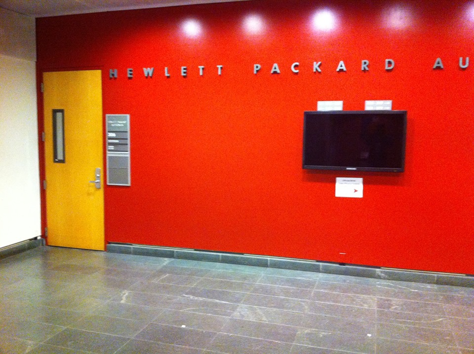
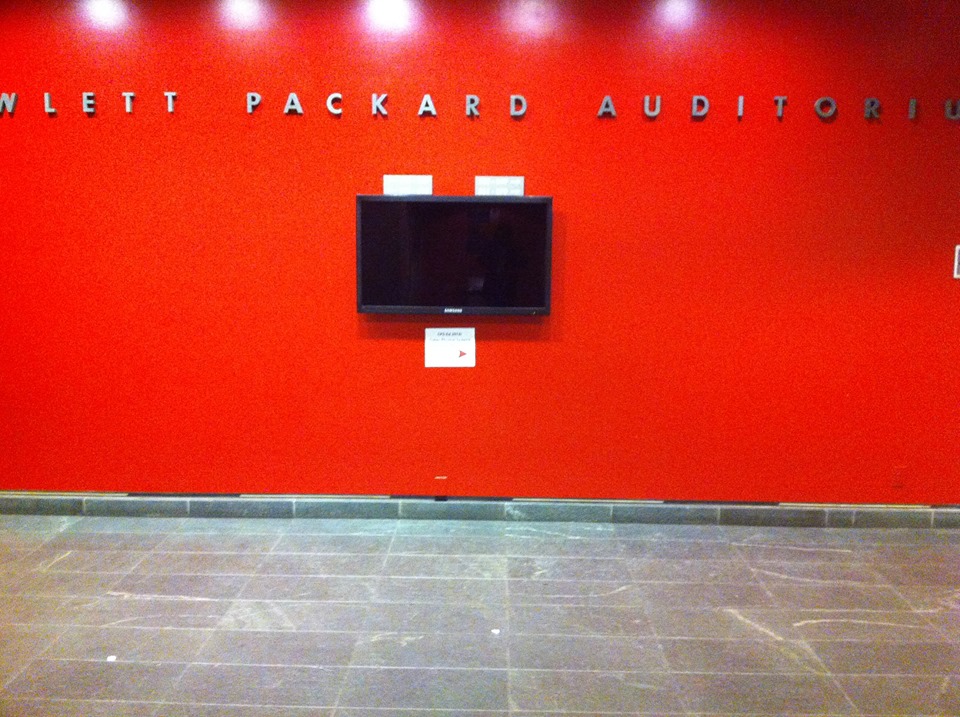
I learned that homography transformations are really cool, and actually not at all mathematically complex. It really does come down to a simple matrix multiplication. I was mostly surprised at how accurate image rectification can really be, and especially how it can be used to view shapes and drawings from completely different angles, offering new perspectives on elements of our visible world!

Bells and Whistles

I was able to find the focal length of my camera in pixels by using information from the EXIF data tags, then fine-tuning the resulting value until my images looked best. The final value used in my code was f = 450 pixels.

1. Cylindrical Mapping

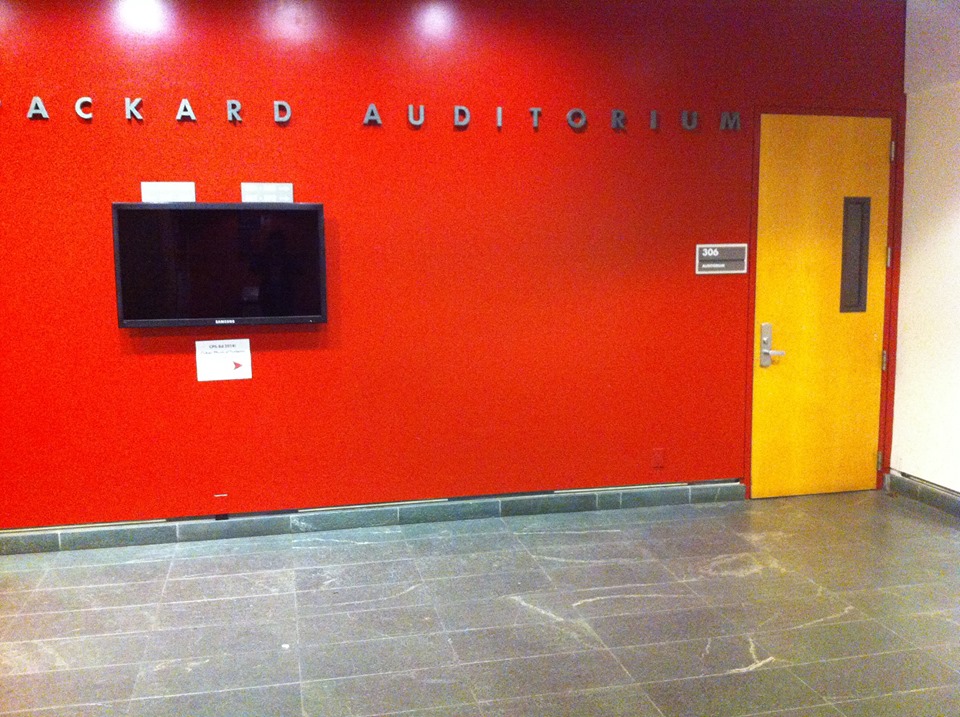
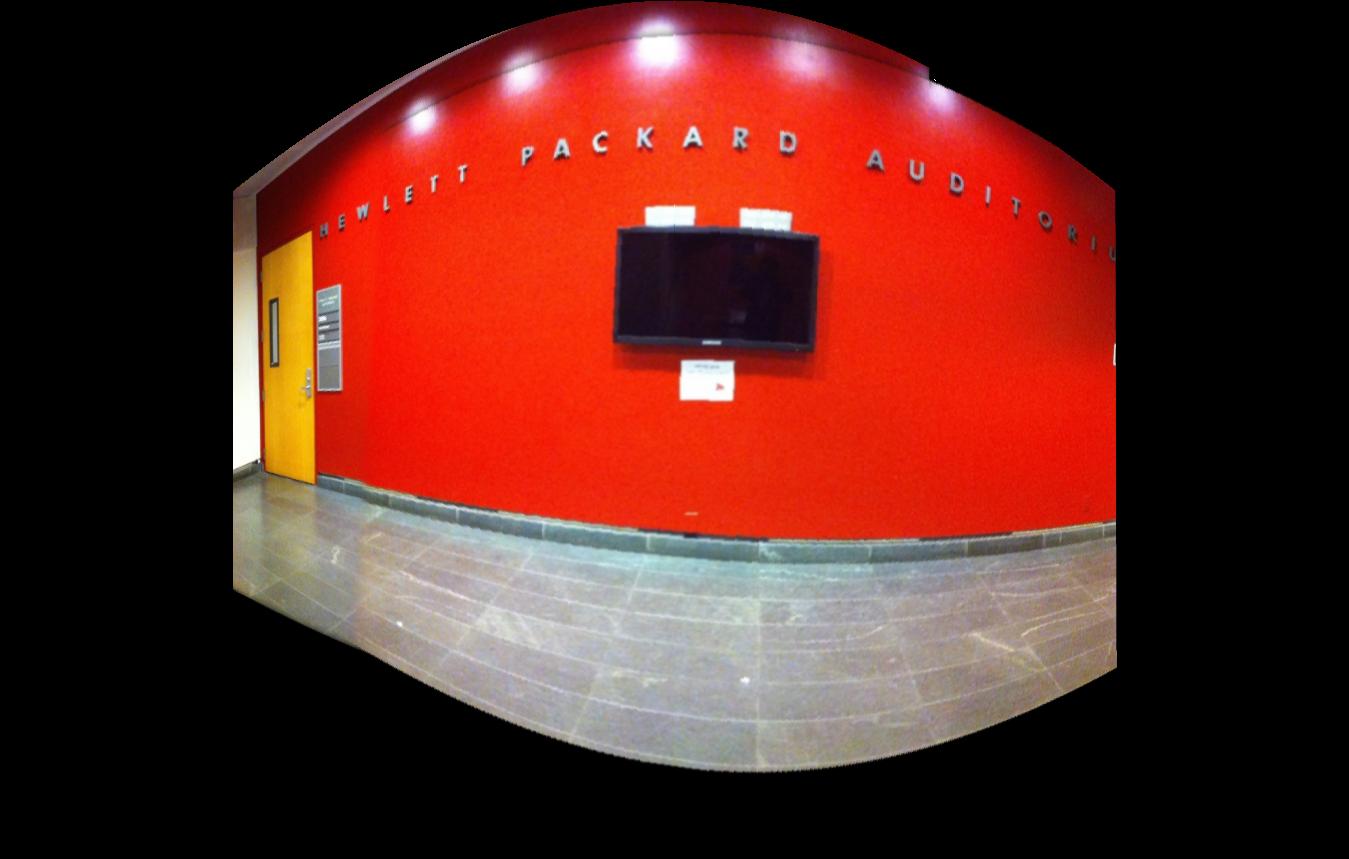
I implemented cylindrical mapping, projecting my mosaic onto a cylinder instead of a plane! To do this, I simply followed the transformation equations presented in class. Here are the results!

Left: The mosaic outside HP Auditorium projected onto a cylinder.

Right: The mosaic of my research lab projected onto a cylinder.

2. 3D Rotational Model

This part actually took me around 15-20 hours to implement........but I'm happy to say that I finally got it working. Basically, in the 3D rotational model, we exploit the fact that only a rotation takes place among pairs of our point correspondences, and so we can compute the optimal rotation matrix using some axis-angle representation math. We start with the observation that H = K * R * K^-1, where K is the camera intrinsic matrix with optical center (0, 0) and R is the rotation matrix between the points. (This assumption about the camera optical center being at the origin turns out to not affect the final result.) We begin with an estimate of R; in my code, I used the identity matrix. Then, we must apply an incremental update to the rotation matrix, by doing R = R_update * R. We continue this iterative procedure until the change to R is very miniscule. To find R_update, we exponentiate omega_cross using the expm function. w_cross is simply the cross product matrix times the vector of omegas, which can be determined using the Jacobian found in the book. Note here that omega basically encodes the direction and magnitude of the rotation, and so is the parameter of the axis-angle representation of the rotation of R.

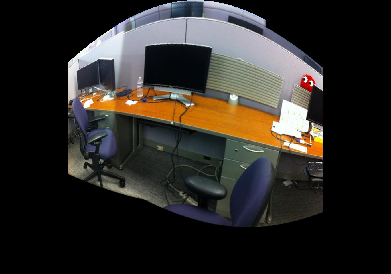
All this took me a long time to implement and debug, but I finally got some neat results. The transformation is a lot more crisp using this method than using a homography transform.

Resulting warps using the 3D rotational model.

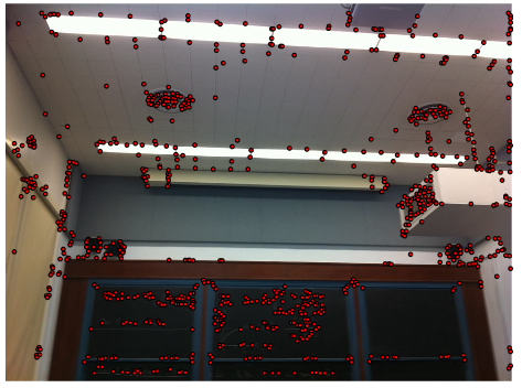
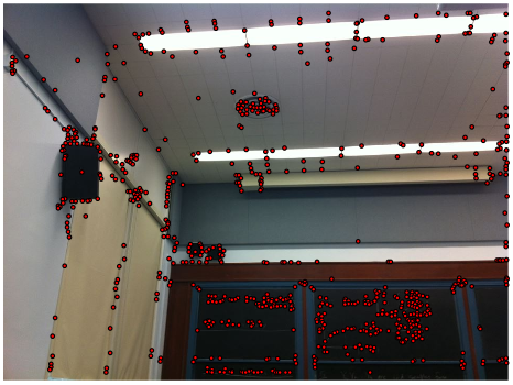
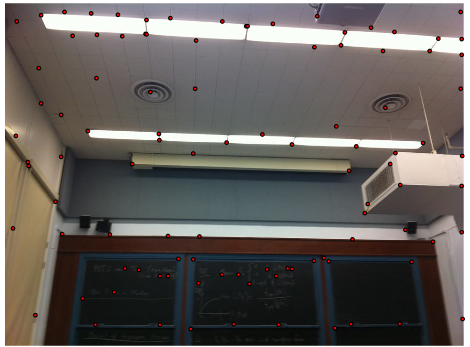
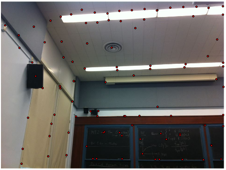
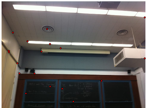
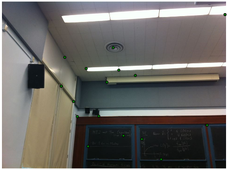
3. Automatic Control Points and Alignment (Done for Part A!)

I was getting super bored of putting in my own control points, so I decided to automate this process! I performed the following steps. First, I implemented my very own Harris corner detector (no built-in library!) and used it on each image. I then used a technique called adaptive non-maximal suppression to only keep a nearly uniformly distributed subset of the chosen points for each image. After, I assigned each point a feature: pixels sampled from the 40x40 grid around that point. Next, I matched points in each image using these features. Finally, I used 4-point RANSAC to compute a good, robust homography matrix not affected by outliers/noise! The results are quite amazing!

Harris points of interest for each image.

Points of interest after filtering using adaptive non-maximal suppression.

The automatically determined control points in each image.

Final mosaic, just as beautiful as before!!!